Learning Objectives
- Define and recognize a population as a group of interacting individuals who are members of the same species, a community as a set of species that interact with each other, and an ecosystem as organisms in a community interacting with each other and with the non-living components in their environment, such as lakes, rivers, mountains, soil, rainfall, etc.
- Name and recognize ecosystems and the biotic (living) and abiotic (non-living) factors that impact where and how organisms live.
- Know the named detrimental (–) / beneficial (+) interactions, including that predation, parasitism, and herbivory are enemy/victim interactions, and recognize examples of them.
- Identify how changes to climate (temperature and precipitation) affect the habitat locations and ranges of biomes.
- Explain biomagnification of toxins through non-linear accumulation of the toxins in higher trophic levels of a food chain.
- Recognize food webs as the feeding interactions between species and predict the outcome if a species in a food web (trophic) disappears or increases dramatically in population.
An ecosystem is a collection of interacting “biotic” or living elements and “abiotic” or non-living elements. Abiotic factors strongly influence where and how organisms live on Earth. Globally, rainfall and temperature are the abiotic factors that define the Earth’s biomes. The heat from sunlight and moisture from the oceans actually drives these patterns by functioning as a very, very large heat engine (refer to the Hadley Cell Cross-Section figure below). Sunlight input at the equator heats the water and air along the equator, generating the numbered cycle below, where the numbers match the diagram:
- Water becomes water vapour and rises with the heated air to up into the atmosphere.
- The rising air cools, causing precipitation in equatorial regions. The warm, now dry air is pushed out of the way by the expanding hotter air below.
- Once it cools, the dry air falls back to earth; because its dry there’s little rain with the air.
- The falling air creates a high pressure area, so surface air redistributes toward locations of lower pressure, such as the equator.
The entire cycle establishes two conveyor belts of air called Hadley cells.
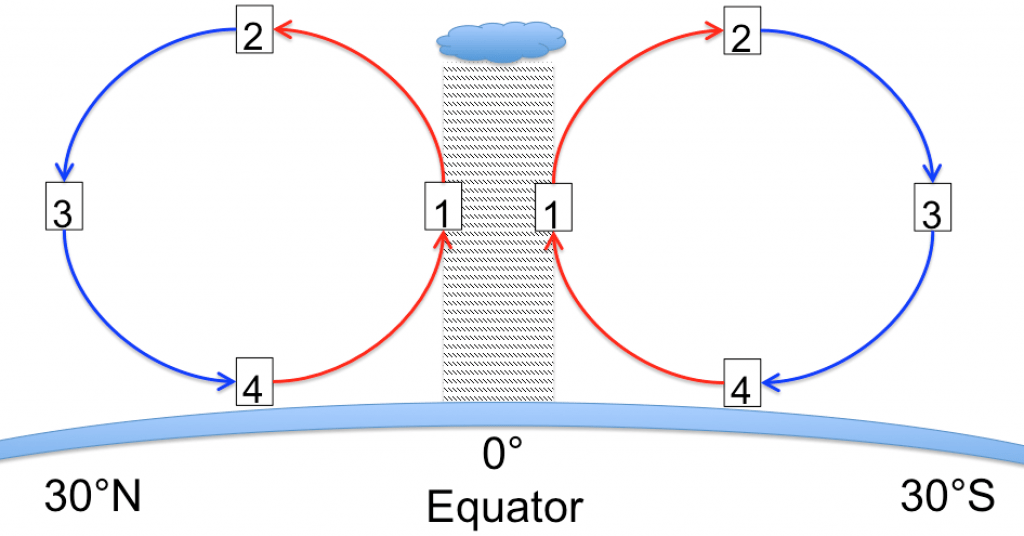
Earth cross-section, showing both Hadley cells, one north of and one south of the equator, and high rainfall levels at the equator. CC-BY by Chrissy Spencer.
Study Tip: Determine where the planet’s cross section fits into the atmospheric cross section above (then read on to the next figure).
The Hadley cells cause bands of wet area at the equator and bands of dry areas at 30 degrees north and south. Notice on the terrestrial biome map below that the equator has wet biomes, like tropical wet forest, while the bands 30 degrees north and south contain the world’s great deserts, among them the Sahara in the northern hemisphere and the deserts of Australia.
Biomes can be aquatic, or marine, as well as terrestrial (shown below), with desert being one example of a common terrestrial biome.
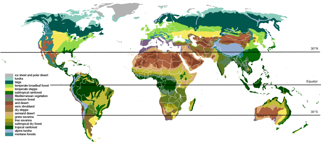
The main biomes of the world. Modified from image by Ville Koistinen (CC BY-SA 3.0, 2007).
This map of biomes allows us to see global ecosystem patterns, such as how deserts or forests are organized with respect to latitude. Interruptions to this pattern occur when major geologic features run counter to latitude. For example, in western South America the biomes run north-to-south instead of east west. The shift is caused by the high-elevation Andes mountain range, which runs along the western coast and disrupts east-west patterns. The mountains’ height disrupts the east-to-west climate patterns more readily evident in Africa and Australia.
If we plot biomes along axes of temperature and precipitation, then we can use graphical organization to predict how environmental changes can alter the biome found in a specific location.
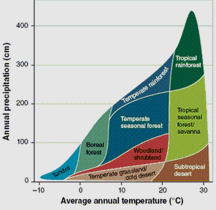
Some common biomes graphed by temperature and precipitation. (Image source: commons.wikimedia.org/wiki/File:PrecipitationTempBiomes.jpg)
For instance, if a wet tundra biome experiences an increase in average annual temperature, what biome would you predict that location to shift to over time?
In biomes governed by water, precipitation matters less while temperature and winds take on a more dominant role. One example of this is ocean upwelling, depicted in the figure below.
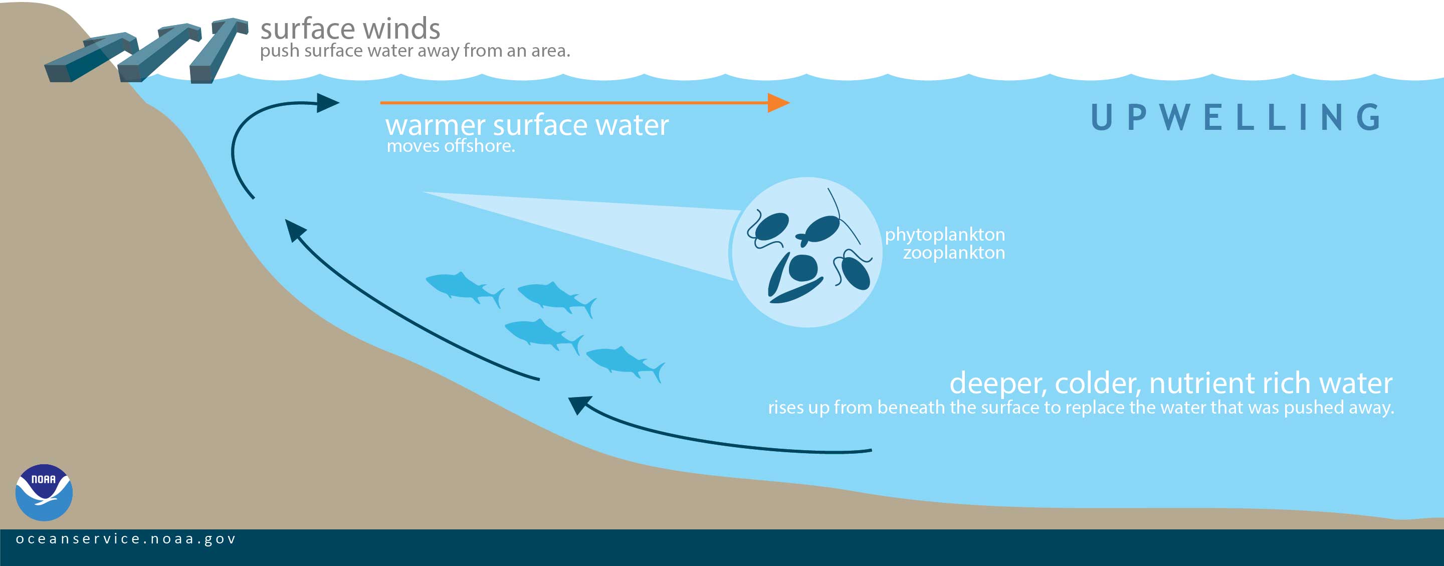
Ocean upwelling (Source: NOAA https://aambpublicoceanservice.blob.core.windows.net/oceanserviceprod/facts/upwelling.jpg)
In the figure, ocean upwelling recycles nutrients in the ocean. Wind (upper/green arrows) blows offshore and displaces surface waters. Waters from the ocean bottom (lower/red arrows) move to the surface in a process called upwelling, bringing with them nutrients from the ocean depths. Why are there nutrients at the bottom of the ocean? When ocean dwelling organisms die, they sink to the bottom, sequestering to the bottom of the ocean all of the nutrients, such as chemical elements, their bodies contain: carbon, nitrogen, oxygen, hydrogen, etc.
Unlike the sunlight energy that powers the heat-engine of the planet, the nutrients on Earth are finite and reusable. Nutrients like phosphorous, nitrogen, and even carbon are the matter on the planet, and this matter cycles through biotic and abiotic locations. For example, in the ocean in the figure above, carbon is in the living organisms, and when those organisms die that carbon falls to the ocean bottom, where biotic activity in the absence of sunlight is much reduced compared to near the surface. Upwelling can bring the carbon back into biotic circulation. Alternatively, the carbon can remain at the bottom and eventually become incorporated into abiotic sedimentary rock. The carbon in rock will be out of circulation until erosion, geologic activity, or human activity like drilling or mining brings it to the surface.
Nutrients can cycle between living organisms when organisms eat each other. Predation or herbivory (enemy-victim interaction) is an obvious way to gain energy for organisms that cannot make their own energy via photosynthesis from the sun. We can depict the movement of energy gained from enemy-victim interactions in a diagram called a food chain, seen below.
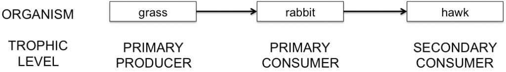
A simple terrestrial food chain shows how energy moves from the eaten to the eater as a rabbit eats grass, and then is eaten by a hawk. Each level of consumption is called a trophic level and is labeled by the species trophic function in the ecosystem (CC-BY by C. Spencer.)
In a food chain, the direction of the arrows indicate the direction of the flow of energy. Most species feed on a variety of prey and plants—obviously a hawk is able to catch other prey in addition to rabbits, and those other prey, say mice, could also eat grass. So, the simple food chain above is oversimplified, and in fact the concept of a food chain itself is too simple for most ecosystems. Instead, a web of feeding patterns better reflect the ways that most species interact in an ecosystem. The basic food web shown below includes the grass-rabbit-hawk food chain, as well as other species at the three trophic levels.
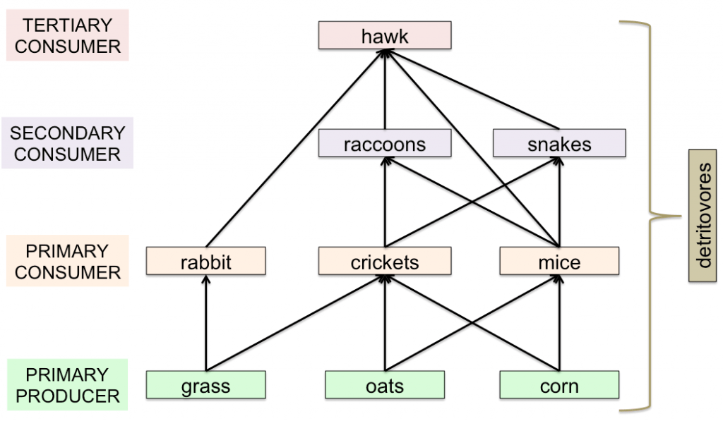
A simple terrestrial food web, where several species occupy each trophic level in a community of interactions. All of the organisms would also have an arrow flowing to detritovores, which are the decomposers of dead organic matter in the ecosystem. (Image Credit: Chrissy Spencer, CC-BY.)
As with the food chain, the arrows show the direction of energy transfer. Every species should also have an additional arrow flowing to the detritivores to indicate the flow of energy upon death (those arrows aren’t shown but are indicated by the bracket). Ecologists use food webs to ask about dependencies between species. In the diagram above, if the hawk population become critically small, what impact would that have on the rest of the ecosystem?
Organisms gain energy through food web dynamics, but there is a potentially detrimental environmental consequences of eating others in contaminated environments: biomagnification. Biomagnification is the increase in concentration of persistent, toxic substances in organisms at each trophic level, from the primary producers to the top consumers. While organisms are very inefficient at acquiring energy through food (on average 10% of the energy is available to the eater), all of the toxins are retained by the eater, often stored in fat or tissue, or trapped in the liver or kidneys. Individual organisms accumulate toxins over their lifetimes.
Substances like DDT, a once common pesticide that bioaccumulated in birds and caused their eggshells to thin, led to high offspring mortality. As a result of the work of biologist and writer Rachel Carson and others, the use of DDT was banned in the United States in the 1970s. Other substances that bioaccumulate are heavy metals like mercury, lead, and cadmium, as well as PCBs. PCBs were banned in 1979 in the US from use in coolant liquids. The figure below shows an example of PCB biomagnification in the Saginaw Bay of Lake Huron:
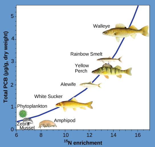
Fish in the higher trophic levels accumulate more PCBs than those in lower trophic levels. PCB concentrations increase more than the linear expectation (shown by tracking naturally occurring heavy isotopes of nitrogen) for accumulation when moving up trophic levels in the Saginaw Bay ecosystem of Lake Huron. The faster-than-linear increase is called biomagnification. (credit: Patricia Van Hoof, NOAA, GLERL)
In class, we’ll consider what could happen to the ecosystem if biomagnification or other changes to the food web occur.
Hank Green’s Crash Course on Ecosystem Ecology summarizes these topics in a quick 10 minute lecture:
Ideas and text on this page include content from Open Stax Biology and the bio1510.biology.gatech.edu online textbook.